Finite-sample analysis of $M$-estimators via self-concordance, II

This is the second of two posts where I present our recent work with Francis Bach on the optimal finite-sample rates for $M$-estimators. Recall that in the previous post, we have proved the Localization Lemma which states the following: stability of the empirical risk Hessian $\mathbf{H}_n(\theta)$ on the Dikin ellipsoid with radius $r$, \[ \mathbf{H}_n(\theta) \asymp \mathbf{H}_n(\theta_*), \, \forall \theta \in \Theta_{r}(\theta_*), \] guarantees that once the score $\Vert\nabla L_n(\theta_*) \Vert_{\mathbf{H}^{-1}}^2$ reaches $\Vert\nabla L_n(\theta_*) \Vert_{\mathbf{H}^{-1}}^2 \lesssim r^2,$ one has the desired excess risk bound: \[ L(\widehat \theta_n) - L(\theta_*) \lesssim \Vert\widehat \theta_n - \theta_*\Vert_{\mathbf{H}}^2 \lesssim \Vert\nabla L_n(\theta_*) \Vert_{\mathbf{H}^{-1}}^2. \] I will now show how self-concordance allows to obtain such guarantees for $\mathbf{H}_n(\theta)$.

Self-concordance

Recall that $\ell(y,\eta)$ is the loss of predicting a label $y \in \mathcal{Y}$ with $\eta = X^\top \theta \in \mathbb{R}$. We assume that $\ell(y,\eta)$ is convex in its second argument, and introduce the following definition:

Definition 1. The loss $\ell(y,\eta)$ is self-concordant (SC) if for any $(y,\eta) \in \mathcal{Y} \times \mathbb{R}$ it holds \[ \boxed{ |\ell'''_\eta(y,\eta)| \le [\ell''_\eta(y,\eta)]^{3/2}. } \]

While the above definition is homogeneous in $\eta$, the next one is not, since the power $3/2$ is removed:

Definition 2. The loss $\ell(y,\eta)$ is pseudo self-concordant (PSC) if instead it holds \[ \boxed{ |\ell'''_\eta(y,\eta)| \le \ell''_\eta(y,\eta). } \]

The first definition is inspired by [3] where similar functions (in $\mathbb{R}^d$) were introduced in the context of interior-point algorithms. As we are about to see, the homogeneity of this definition in $\eta$ allows to qualify the precision of local quadratic approximations of empirical risk in affine-invariant manner, which is a natural requirement if we recall that $M$-estimators are themselves affine-invariant. This is violated in the second definition; will see that this leads to the increased sample size to guarantee the optimal excess risk for PSC losses, under the extra assumption. On the other hand, PSC losses are somewhat more common. I will now give several examples of SC and PSC losses.

1. One family of examples arises in generalized linear models (GLMs). In particular, the logistic loss \[ \ell(y,\eta) = \frac{\log(1 + e^{-y\eta})}{\log 2}, \] is PSC (see [4]). In fact, one can consider other GLM losses with canonical parameter, given by \[ \ell(y,\eta) = - y\eta + a(\eta) - b(y), \] where the cumulant $a(\eta)$ can be written as \[ a(\eta) = \mathbb{E}_{p_\eta}[Y] \] where $ p_\eta(y) \propto e^{y\eta + b(y)} $ is the density that the model imposes on $Y$. Thus, for GLMs self-concordance can be interpreted in terms of this model distribution of $Y$: for $s \in \{2,3\}$ we have \[ \ell_\eta^{(s)}(y,\eta) = a^{(s)}(\eta) = \mathbb{E}_{p_\eta} [(Y - \mathbb{E}_{p_\eta}Y)^s]. \] Then, (pseudo) self-concordance specifies the relation between the central moments of $p_\eta(\cdot)$. In particular, we see that the logistic loss is PSC simply because $\mathcal{Y} = \{0,1\}$, and hence \[ |a'''(\eta)| \le \mathbb{E}_{p_\eta} |(Y - \mathbb{E}_{p_\eta}[Y])^3| \le \mathbb{E}_{p_\eta} [(Y - \mathbb{E}_{p_\eta}[Y])^2] = a''(\eta). \] Another example of a PSC loss arises in Poisson regression where the model assumption is that $Y \sim \text{Poisson}(e^\eta)$ which corresponds to $a(\eta) = \exp(\eta)$. Unfortunately, this implies heavy-tailed distribution of the calibrated design $\tilde X(\theta)$ under the model distribution which creates additional difficulties – see our paper for more details.

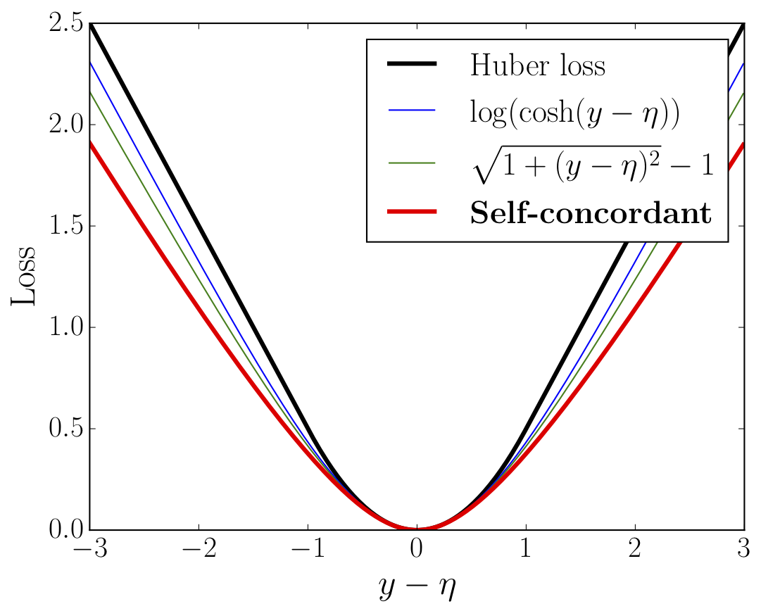
2. Another family of PSC losses arises in robust estimation. Here, $\ell(y,\eta) = \varphi(y-\eta)$ with $\varphi(\cdot)$ being convex, even, 1-Lipschitz, and satisfying $\varphi''(0) = 1$. The prototypic example of a robust loss is the Huber loss corresponding to \[ \varphi(t) = \left\{ \begin{align} &{t^2}/{2}, &\quad|t| &\le 1, \
   &\tau t - 1/2, &\quad |t| &> 1. \end{align} \right. \] However, $\varphi'''(t)$ doesn’t exist at $t = \pm 1$, so it is not SC nor PSC. Fortunately, the Huber loss can be well-approximated by some pseudo-Huber losses that turn out to be PSC (see the figure below): \begin{align} \label{def:pseudo-huber} \varphi(t) &= \log\left(\frac{\exp(t) + \exp(-t)}{2}\right), \
   \varphi(t) &= \sqrt{1 + {t^2}}-1. \end{align}

3. Finally, we can construct SC losses using the classical result from [3] that self-concordance is preserved under taking the Fenchel conjugate.

   The Fenchel conjugate of a self-concordant function $\varphi^*: D \to \mathbb{R}$, where $D \subseteq \mathbb{R}$, is also self-concordant.

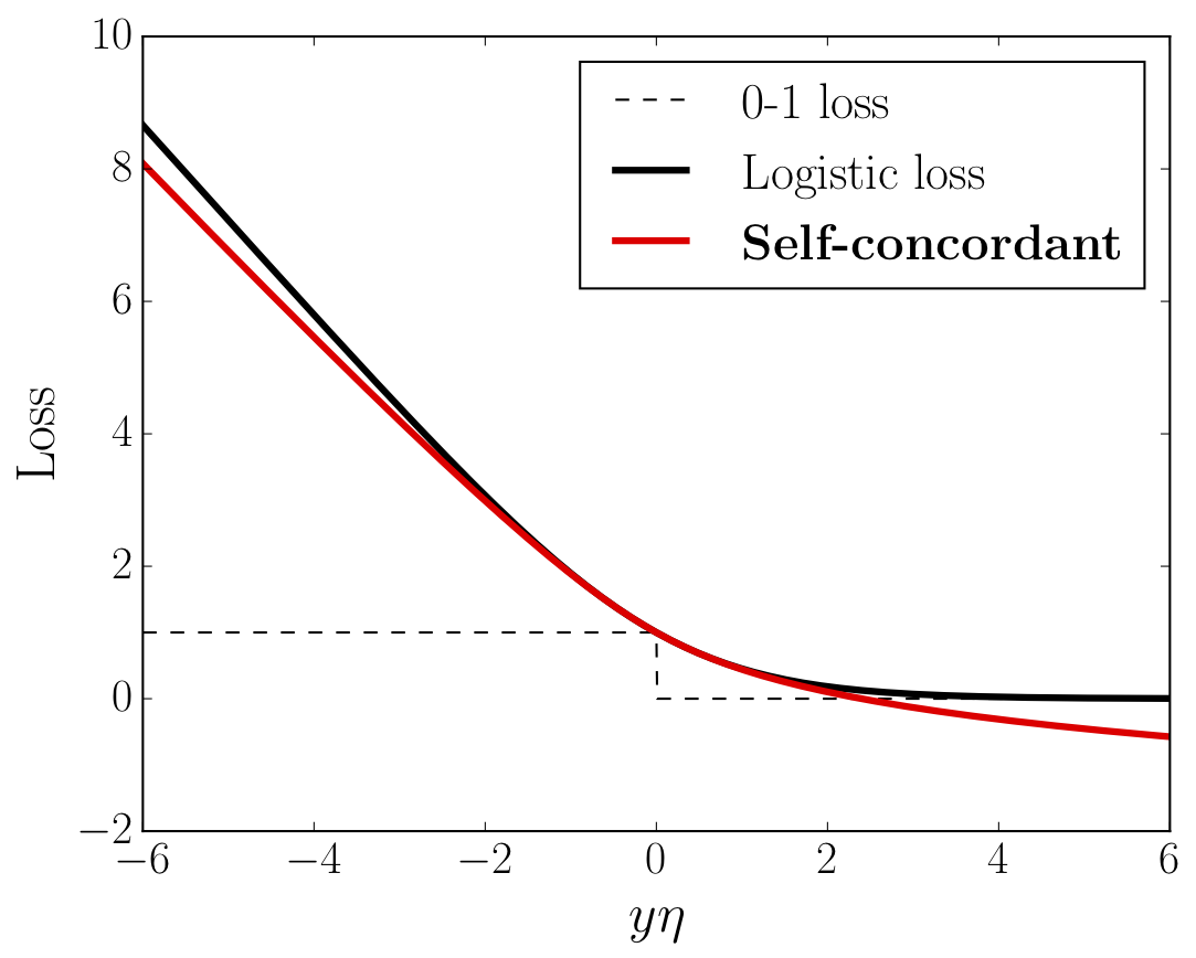
This fact allows to construct SC losses with derivatives ranging over a given interval, by computing the convex conjugate of the logarithmic barrier of a given subset of $\mathbb{R}$. In particular, taking the log-barrier on $[-1,1]$, we obtain an analogue of Huber’s loss, and the log-barrier on $[-1,0]$ results in the analogue of the logistic loss (see the figure below). Note that in the latter case, our loss does not upper bound for the 0-1 loss. However, its negative part grows as a logarithm, and using the well-known calibration theory from (Bartlett et al., 2006), one can show that the related expected risk still well-approximates the probability of misclassification.

Integration argument and the basic result

By the Localization Lemma, our task reduces to proving that the empirical Hessian is stable, with high probability, in the Dikin ellipsoid $\Theta_r(\theta_*)$ with a constant radius $r$. On the other hand, self-concordance easily allows to get \[ r = O\left(\frac{1}{\sqrt{d}}\right) \] using a simple integration technique sketched below. This leads to the bound \[ n \gtrsim d \cdot d_{eff}, \] up to the dependency on $\delta$ and subgaussian constants.

1. Indeed, let the loss be SC, and recall that the Hessian of the empirical risk at point $\theta$ is \[ \mathbf{H}_n(\theta) = \frac{1}{n} \sum_{i=1}^n \ell''(Y_i,X_i^\top\theta) X_i X_i. \] Hence, we can compare $\mathbf{H}_n(\theta)$ with $\mathbf{H}_n(\theta_*)$ by comparing $\ell''(Y_i,X_i^\top\theta)$ with $\ell''(Y_i,X_i^\top\theta_*)$.

2. Integrating $|\ell'''(y,\eta)| \le [\ell''(y,\eta)]^{3/2}$ from $\eta_* = X^\top \theta_*$ to $\eta = X^\top \theta$, we arrive at \[ \frac{1}{(1+[\ell''(y,\eta_*)]^{1/2}|\eta - \eta_*|)^2} \le \frac{\ell''(y,\eta)}{\ell''(y,\eta_*)} \le \frac{1}{(1-[\ell’‘(y, \eta_*)]^{1/2}|\eta - \eta_*|)^2}, \] or equivalently, \[ \frac{1}{(1+|\langle \tilde X(\theta_*), \theta - \theta_* \rangle|)^2} \le \frac{\ell''(Y,X^\top \theta)}{\ell''(Y,X^\top \theta_*)} \le \frac{1}{(1- |\langle \tilde X(\theta_*), \theta - \theta_* \rangle|)^2}. \] 3. The ratio is bounded if $|\langle \tilde X(\theta_*), \theta-\theta_* \rangle| \le c < 1$. By Cauchy-Schwarz, it suffices that \[ \Vert\tilde X(\theta_*)\Vert_{\mathbf{H}(\theta_*)^{-1}} \Vert(\theta-\theta_*)\Vert_{\mathbf{H}(\theta_*)} \le c. \] On the other hand, $\mathbf{H}(\theta_*)^{-1/2}\tilde X(\theta_*)$ is a $K_2$-subgaussian vector in $\mathbb{R}^d$, therefore, \[ \Vert\tilde X(\theta_*)\Vert_{\mathbf{H}(\theta_*)^{-1}} = \Vert\mathbf{H}(\theta_*)^{-1/2} \tilde X(\theta_*)\Vert_{2} = O(K_2\sqrt{d}). \] Thus, we can guarantee that with high probability, $\mathbf{H}_n(\theta) \asymp \mathbf{H}_n(\theta_*)$ for any $\theta$ such that \[ \Vert(\theta-\theta_*)\Vert_{\mathbf{H}(\theta_*)} \le \frac{c}{K_2 \sqrt{d}}, \] i.e., in the Dikin ellipsoid $\Theta_r(\theta_*)$ with radius $r \lesssim \frac{K_2}{\sqrt{d}}$. Combining this with the Localization Lemma and some union bounds, we obtain the following result:

Theorem 1. Assume that the loss is self-concordant, and $\mathbf{G}^{-1/2}\nabla \ell_\theta(Y,X^\top \theta_*),$ $\mathbf{H}^{1/2}\tilde X(\theta_*)$ are, correspondingly, $K_1$- and $K_2$- subgaussian. Then, with probability at least $1-\delta$ it holds \[ \label{eq:main-ineq} \boxed{ L(\widehat\theta_n) - L(\theta_*) \lesssim \Vert\widehat\theta_n - \theta_*\Vert_{\mathbf{H}}^2 \lesssim \frac{K_1^2 d_{eff} \log(1/\delta)}{n} } \] provided that \begin{equation} \label{eq:n-mine-complex} \boxed{ n \gtrsim \max\left\{K_2^4 \left( {\color{blue} d} + \log\left(1/\delta\right)\right), \; {\color{red} d} K_1^2 K_2^2 {\color{blue}{d_{eff}}}\log\left(d/{\delta}\right)\right\}. } \end{equation}

We see that the critical sample size grows as the product of $d_{eff}$ and $d$, since we can only guarantee that $\mathbf{H}_n(\theta)$ is stable in the small Dikin ellipsoid with $O(1/\sqrt{d})$ radius. In fact, this result can be improved. But before showing how this can be achieved, let me consider the case of PSC losses.

Pseudo self-concordant losses

In the case of PSC losses, a integration argument – but this time integrating $|\ell'''(y,\eta)| \le \ell''(y,\eta)$ – implies that in order to bound the ratio of the second derivatives, we must ensure that \[ \Vert X\Vert_{\mathbf{H}^{-1}} \Vert(\theta-\theta_*)\Vert_{\mathbf{H}}\le c, \] that is, the calibrated design $\tilde X(\theta_*) = [\ell''_\eta(Y,X^\top \theta_*)]^{1/2}X$ gets replaced with $X$. Intuitively, this is due to the lack of the extra square root of $\ell''_\eta(y,\eta)$ in Definition 2. To control $\Vert X\Vert_{\mathbf{H}(\theta_*)^{-1}}$, we can introduce the standard assumption from [4], relating $\mathbf{H}(\theta_*)$ and the second-moment matrix of the design, $\boldsymbol{\Sigma} := \mathbb{E}[X X^\top]$, as follows: \[ \boldsymbol{\Sigma} \preccurlyeq \rho \mathbf{H}. \] By a similar argument, we show that under this additional assumption, and assuming that $\boldsymbol{\Sigma}^{-1/2}X$ is $K$-subgaussian, the critical sample size from Theorem 1 gets replaced with \begin{equation} \label{eq:n-fake-complex} \boxed{ n \gtrsim \max\left\{K_2^4 \left(\color{blue}{d} + \log\left({1}/{\delta}\right)\right), \; \color{red}{\rho d} K^2 K_1^2 \color{blue}{d_{eff}} \log\left(d/{\delta}\right)\right\}; } \tag{PSC} \end{equation} essentially, it becomes $\rho$ times larger. Note that the only generic upper bound available for $\rho$ is \[ \rho \le \frac{1}{\inf_{\eta} \ell''_{\eta}(y,\eta)}, \] where $\eta$ ranges over the set $\left\{\eta(\theta) = X^{\top} \theta, \;\theta \in \Theta \right\},$ and $\Theta$ is the set of possible predictors. In particular, in logistic regression with $\Vert X \Vert_2 \le D$ and $\Theta = \{\theta \in \mathbb{R}^d: \Vert\theta\Vert_2 \le R\}$, this gives \[ \rho \lesssim \exp({RD}). \] Moreover, this bound is achievable on a certain (quite artificial) distribution of $X$ as shown in (Hazan et al., 2014). However, the actual value of $\rho$ depends on the data distribution, and is moderate when this distribution is not chosen adversarially as discussed in (Bach and Moulines, 2013). In fact, in the paper we show that in logistic regression with Gaussian design $X \sim \mathcal{N}(0, \boldsymbol{\Sigma})$ one has \[ \rho \lesssim 1+\Vert\theta_*\Vert_{\boldsymbol{\Sigma}}^3. \] Still, $\rho \gg 1$ when $\Vert\theta_*\Vert_{\boldsymbol{\Sigma}} \gg 1$, and our construction of self-concordant analogues of the Huber and logistic losses remains useful.

Near-linear bounds via a covering argument

In fact, we can get rid of the extra $O(d)$ factor in the previous bounds for the critical sample size, and obtain the bounds that scale near-linearly in $\max(d, d_{eff})$. In particular, in the case of self-concordant losses the critical sample size in the case of SC losses can be reduced to \begin{equation} \label{eq:n-mine-improved} \boxed{ n \gtrsim \max\left\{\bar K_2^4 d\log\left({d}/\delta\right), \; K_1^2 \bar K_2^6 d_{eff} \log\left(1/\delta\right)\right\}. } \tag{SC$^*$} \end{equation} This is done via a more delicate argument, as explained below, and under the mild extra assumption that the calibrated design $ \tilde X(\theta) $ is $\bar K_2$-subgaussian, when multiplied by $\mathbf{H}(\theta)$, at every point $\theta$ of the unit Dikin ellipsoid $\Theta_1(\theta_*)$, with $\bar K_2$ independent of $\theta$. For pseudo self-concordant losses, the second bound gets inflated by $\rho$; on the other hand, the radius of the Dikin ellipsoid in which $\tilde X(\theta)$ is required to be uniformly subgaussian decreases by the factor of $1/\sqrt{\rho}$. In fact, the extra assumption appears to be essetial. For example, in the paper we show that in logistic regression with $X \sim \mathcal{N}(0,\boldsymbol{\Sigma})$, one has \[ \bar K_2 \lesssim K_2 + 1, \] where $K_2$ is the subgaussian constant of $\mathbf{H}(\theta_*)^{-1/2}\tilde X(\theta_*)$, and the two assumptions are equivalent.

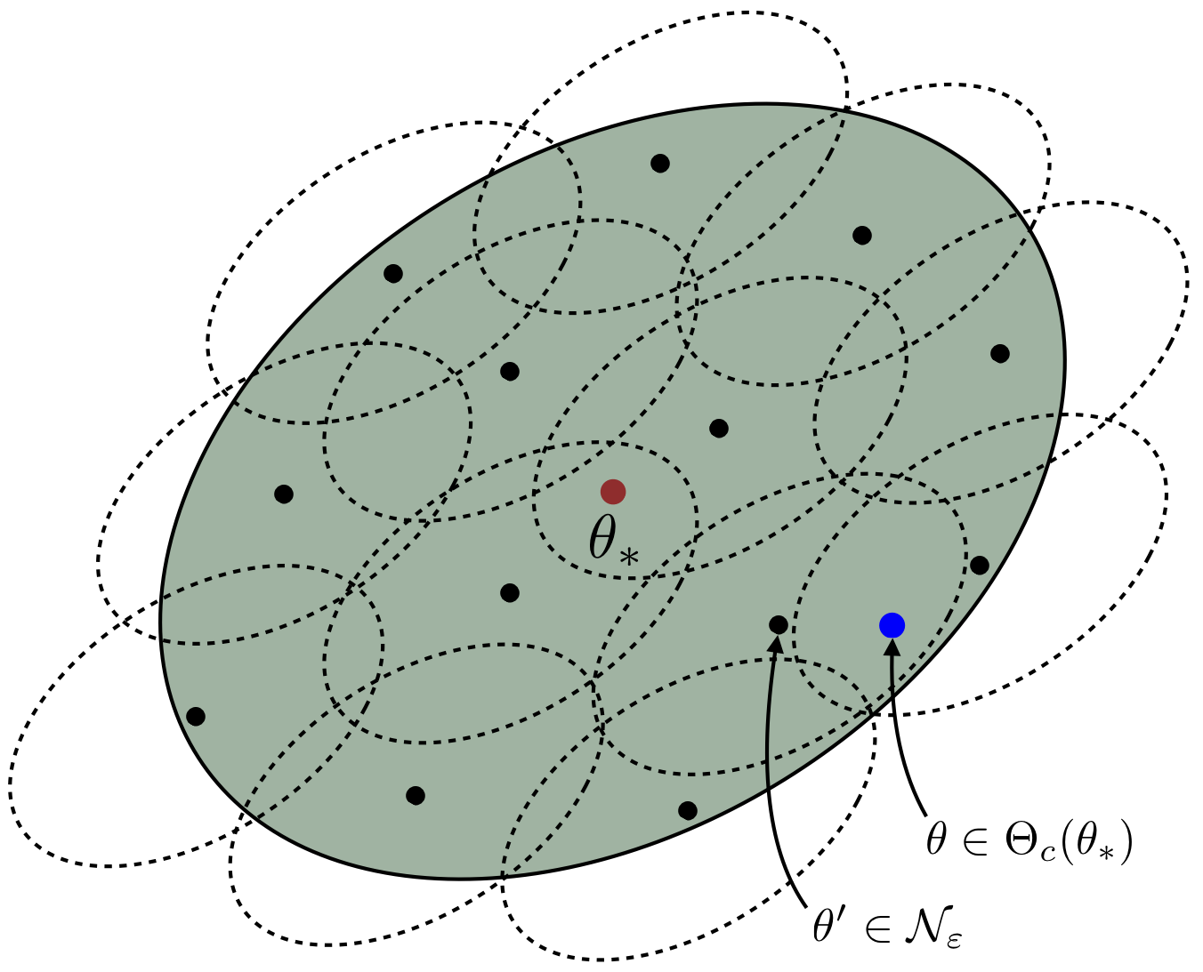
Let us briefly explain the main ideas behind the proof of the improved bounds (see the figure above). First of all, recall that the extra $d$ factor in the previous bounds appeared because we used self-concordance of the individual losses, which only allowed to prove stability of the empirical Hessian in a small Dikin ellipsoid with radius $O(1/\sqrt{d})$. This factor would be eliminated if we managed to show a probabilistic bound \[ \mathbf{H}_n(\theta) \asymp \mathbf{H}_n(\theta_*), \] uniformly over the Dikin ellipsoid $\Theta_{c}(\theta_*)$ with a constant radius. Such bound could have been obtained via an integration argument, should we have self-concordance of $L_n(\theta)$. However, unlike the individual losses, the empirical risk is not self-concordant, we have to come up with a more subtle argument. In a nutshell, this argument combines the following ingredients:

1. Self-concordance of the expected risk $L(\theta)$ on $\Theta_c(\theta_*)$, with $c = 1/\bar K_2^{3/2}$, which follows from the subgaussian assumption about $\tilde X(\theta)$ and the relation between the moments of a subgaussian vector. This guarantees that for any $\theta \in \Theta_c(\theta_*)$ it holds \[ \mathbf{H}(\theta) \asymp \mathbf{H}(\theta_*). \]

2. Self-concordance of the individual losses which guarantees, for any $\theta_0 \in \mathbb{R}^d$ and $\theta \in \Theta_{1/\sqrt{d}}(\theta_0)$, that \[ \mathbf{H}_n(\theta) \asymp \mathbf{H}_n(\theta_0). \]

3. Finally, a covering argument, in which $\Theta_c(\theta_*)$ is covered with smaller $O(1/\sqrt{d})$-ellipsoids. The problem then reduces to the control of the supremum \[ \sup_{\theta_0 \in \mathcal{N}} \Vert \mathbf{H}(\theta_0)^{-1/2} \mathbf{H}_n(\theta_0) \mathbf{H}(\theta_0)^{-1/2}\Vert, \] where $\Vert\cdot\Vert$ is the operator norm, and $\mathcal{N}$ is the epsilon-net corresponding to the covering of $\Theta_c(\theta_*)$. This gives the extra $O(\log d)$ factor in \eqref{eq:n-mine-improved} since $\log(|\mathcal{N}|) = O(d \log d)$.

Conclusion

We have demonstrated how to obtain fast rates for the excess risk of $M$-estimators in finite-sample regimes. Our analysis can handle $M$-estimators with losses satisfying certain self-concordance-type assumptions that hold in some generalized linear models, notably logistic regression, and in robust estimation. These assumptions allow to control the precision of local quadratic approximations for the empirical risk.

One topic that remained beyond the scope of this post is the $\ell_1$-regularized estimators in sparse high-dimensional regimes. There, we have not yet established the improved rates that should scale near-linearly with the sparsity of $\theta_*$. Another possible extension are matrix-parametrized models that arise in covariance matrix estimation and independent component analysis, and application of our techniques to algorithmically efficient procedures such as stochastic approximation.

References

1. B. Laurent and P. Massart. Adaptive estimation of a quadratic functional by model selection. Ann. Statist., 28:5(2000), 1302-1338.

2. V. Spokoiny. Parametric estimation. Finite sample theory. Ann. Statist., 40:6(2012), 2877-2909.

3. A. Nemirovski and Yu. Nesterov. Interior-point polynomial algorithms in convex programming. Society for Industrial and Applied Mathematics, Philadelphia, 1994.

4. F. Bach. Self-concordant analysis for logistic regression. Electron. J. Stat., 4(2010), 384-414.

5. R. Vershynin. Introduction to the non-asymptotic analysis of random matrices. Compressed Sensing: Theory and Applications, 210–268. Cambridge University Press, 2012.

6. D. Hsu, S. Kakade, and T. Zhang. Random design analysis of ridge regression. COLT, 2012.

7. P. Bartlett, M. Jordan, and J. McAuliffe. Convexity, classification, and risk bounds. J. Am. Stat. Assoc., 101:473(2006), 138–156.

8. E. Hazan, T. Koren, and K. Levy. Logistic regression: tight bounds for stochastic and online optimization. COLT, 2014.

9. F. Bach and E. Moulines. Non-strongly-convex smooth stochastic approximation with convergence rate $O(1/n)$. NIPS, 2013.